Zucchetti LLM Course — Lecture 1 of 10

The Transformer
Blueprint

How Large Language Models work under the hood

Deep dive into the architecture

Kamyar Zeinalipour · 2 hours

Today’s Agenda

15 min What is an LLM? Timeline & Key Papers

30 min Transformer Architecture: Attention, Multi-Head, Q/K/V

20 min Encoder vs Decoder & How LLMs Generate Text

25 min Training, Hallucination, Temperature & Sampling

20 min Scale, Perplexity, Context Windows & RLHF

10 min Q&A

Total: 2 hours (120 min) · Deep theory session — hands-on lab in Lecture 2

Section 1 of 4

The Transformer
Blueprint

The architecture that changed everything

What is an LLM, Really?

Think of it as the world's most sophisticated autocomplete

Your phone keyboard:

"See you" → tomorrow | later | soon

An LLM (same idea, but trained on the entire internet):

"Explain quantum computing" → generates a full, coherent answer

What it IS

A statistical model trained on text
Predicts the most likely next word
Very good at patterns and language

What it is NOT

Not a database of facts
Not reasoning from first principles
Not guaranteed to be correct

Before Transformers

RNNs / LSTMs

Process words one by one
Sequential = slow
Long texts → forget the beginning
Hard to parallelize on GPUs

Transformers (2017)

Process all words at once
Parallel = fast
Attention spans the full context
GPU-native architecture

Transformers made it possible to train on trillions of tokens — that's what enabled GPT, LLaMA, and everything we use today.

The Timeline: How We Got Here

2017 📄 "Attention Is All You Need" paper — Transformers invented

2018 BERT (Google) — first big pre-trained language model

2020 GPT-3 (OpenAI) — 175B params, showed emergent abilities

2022 ChatGPT launched — AI goes mainstream

2023 GPT-4, LLaMA 2, Mistral — open-source revolution begins

2024-25 LLaMA 3, Gemini, Claude, DeepSeek — multimodal, agents, reasoning

Everything happened in just 8 years. The Transformer architecture is the single most important invention in modern AI.

The Papers That Built Modern AI

Each paper built on the previous one. Understanding this lineage helps you understand why current models work.

Year	Paper	Key Innovation	Citations
2013	Word2Vec (Mikolov et al.)	Words as vectors — similar meaning = similar direction	35,000+
2017	Attention Is All You Need (Vaswani et al.)	Transformer architecture — parallel attention replaces RNNs	250,000+
2018	BERT (Devlin et al., Google)	Pre-train once → fine-tune for any task	115,000+
2020	GPT-3 (Brown et al., OpenAI)	In-context learning — no fine-tuning needed, just examples	60,000+
2022	InstructGPT (Ouyang et al.)	RLHF — train models to follow human instructions	8,000+
2023	LLaMA (Touvron et al., Meta)	Open-source foundation models — democratized LLMs	12,000+

These 6 papers define the entire field. Everything in this course connects back to them.

The Transformer Architecture

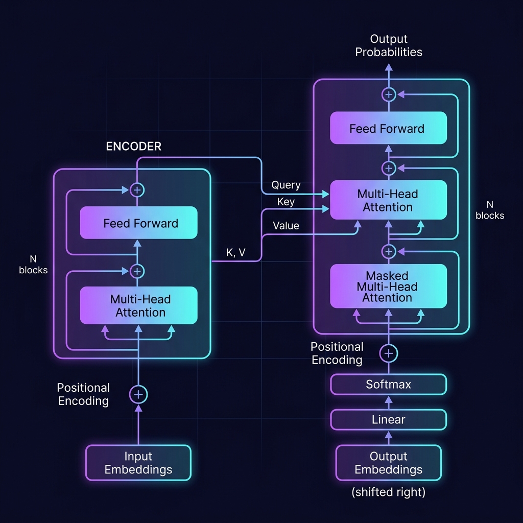
The original architecture from "Attention Is All You Need" (Vaswani et al., 2017)

Running Example — We will trace this sentence through the next 3 slides:
“The bank approved the loan for the new house”
Input text → Encoder blocks → Self-Attention inside each block → rich understanding

Why Position Matters

Transformers process all words at once — they have no idea about word order.

Without position info, these two sentences look identical to the model:

“The dog bit the man” vs “The man bit the dog”

Same words, same embeddings — but completely different meaning!

Solution: add a unique position vector to each word’s embedding:

	Word	Embedding	+	Position	=	Final input x
pos 1	“The”	`[0.10, 0.20]`	+	`[0.00, 1.00]`	=	`[0.10, 1.20]`
pos 2	“dog”	`[0.80, 0.30]`	+	`[0.84, 0.54]`	=	`[1.64, 0.84]`
pos 3	“bit”	`[0.50, 0.60]`	+	`[0.91, −0.42]`	=	`[1.41, 0.18]`

Now “dog” at position 2 has a different vector than “dog” at position 5 — the model can tell them apart!

Each position gets a unique fingerprint. The same word at different positions produces different vectors. Next slide: how these position vectors are computed.

Positional Encoding — The Math

Each position gets a unique vector computed using sine and cosine at different frequencies.

PE(pos, 2i) = sin(pos / 10000^2i/d)

PE(pos, 2i+1) = cos(pos / 10000^2i/d)

Why sin/cos?

Each dimension has a different frequency — like a clock with hands ticking at different speeds
The model can learn relative distances: “3 words apart” always looks the same
Works for sequences longer than training data — no limit!

Modern alternative: RoPE

Rotary Position Embedding — used in LLaMA, Gemini
Instead of adding to embeddings, it rotates the Q and K vectors
Better at handling very long contexts (100K+ tokens)

The final input to the transformer is: x = token embedding + positional encoding. This combined vector is what enters Block 1.

Self-Attention: The Core Idea

Every word asks: “Which other words are relevant to me?”

“The bank approved the loan for the new house”

← “bank” attends to “loan” (financial context, not river bank)
← “loan” attends to “bank” AND “house” (purpose of the loan)

📚 Library Analogy for Q, K, V

Query (Q): “I need info about Italian cooking”
Key (K): Each book's label on the shelf
Value (V): The actual book content inside

Match query against all keys → read best-matching values

In a transformer, every word plays all 3 roles at the same time.

Attention(Q, K, V) = softmax(QK^T / √d_k) · V

softmax turns scores into percentages
√d keeps the numbers from exploding

Q, K, V all come from the same input — next slide: the math with real numbers

Self-Attention: Step-by-Step with Numbers

Let’s trace what happens when “bank” computes its attention scores

The 6 Steps

“The bank approved the loan for the new house”

1.	“bank” Q × “loan” K	4.2
2.	“bank” Q × “house” K	2.1
3.	“bank” Q × “approved” K	1.8
4.	Divide by √d = √3 ≈ 1.73	2.43, 1.21, 1.04
5.	Softmax → percentages	0.40, 0.25, 0.22, ...
6.	Weighted sum of V → new vector

What Just Happened?

The new “bank” vector is now:

40% influenced by “loan”
25% influenced by “house”
22% influenced by “approved”
rest: “The”, “for”, “the”, “new”

The model now knows “bank” means a financial institution — because “loan” had the highest score.

But this was just ONE head. It found the meaning. What about grammar, position, purpose?

The highest Q×K score wins the most influence. “bank” × “loan” = 4.2 (strong match!) → after softmax = 0.40 (40%). Next slide: multiple heads for multiple patterns.

Multi-Head Attention — The Full Picture

One head found “bank↔loan”. But language has many types of relationships. Multiple heads learn different patterns simultaneously.

MultiHead(Q, K, V) = Concat(head₁, ..., headₕ) · W^O

where headᵢ = Attention(Q·Wᵢ^Q, K·Wᵢ^K, V·Wᵢ^V) — each head has its OWN weight matrices

🔗

Head 1: Syntax

bank ↔ approved

subject–verb agreement

🧠

Head 2: Meaning

bank ↔ loan

financial context

📍

Head 3: Position

The ↔ bank

nearby word context

🔙

Head 4: Purpose

loan ↔ house

loan purpose → house

Concat all 4 views → the word “bank” now has a complete understanding of the sentence: it is a financial bank (Head 2), that approved something (Head 1), is the subject (Head 3), related to a house purchase (Head 4).

Inside One Transformer Block

Now you know what attention is. Let’s see where it fits inside the architecture.

What is x? Block 1: x = token embedding + positional encoding | Block 2+: x = output of previous block — each block refines the understanding further

Step 1: Multi-Head Self-Attention

x₁ = x + MultiHeadAttention(LayerNorm(x))

All words look at each other (what we just learned) → + x adds the original back (residual)

⬇️

Step 2: Feed-Forward Network (FFN)

x₂ = x₁ + FFN(LayerNorm(x₁))

Each word independently passes through a small neural network — the “memory” that stores learned facts

⬇️

FFN internally:

FFN(x) = max(0, xW₁+b₁) · W₂+b₂

ReLU activation + two linear layers. LayerNorm stabilizes values. + x is the residual connection.

BERT: 12 blocks, 12 heads, 110M params

GPT-3: 96 blocks, 96 heads, 175B params

One block = attention + FFN. The model stacks N of these. BERT has 12, GPT-3 has 96. Next slide: how Q, K, V are actually created inside Step 1.

How Q, K, V Are Created

The same input passes through 3 different learned lenses

The Expanded Chain

A. LayerNorm(x) → x_norm B. x_norm × W^Q → Q x_norm × W^K → K x_norm × W^V → V C. softmax(QK^T/√d) · V D. x₁ = x + output

W^Q, W^K, W^V = 3 “lenses”

W^Q → “What am I looking for?”

W^K → “What do I contain?”

W^V → “What info do I carry?”

These are learned during training — not hand-coded!

Concrete Trace: “bank”

Input: [0.23, −0.11, 0.55]

A. LayerNorm: [0.21, −0.10, 0.52]

B. × W^Q: Q = [1.2, 0.8]
“looking for financial context”

× W^K: K = [0.9, 1.4]
“I am an institution”

× W^V: V = [0.5, 0.3]
“banking services”

C. Attention: [0.31, −0.08, 0.60]

D. + Residual: [0.54, −0.19, 1.15]

After FFN: [0.48, −0.22, 0.95] ✓

Attention in Action

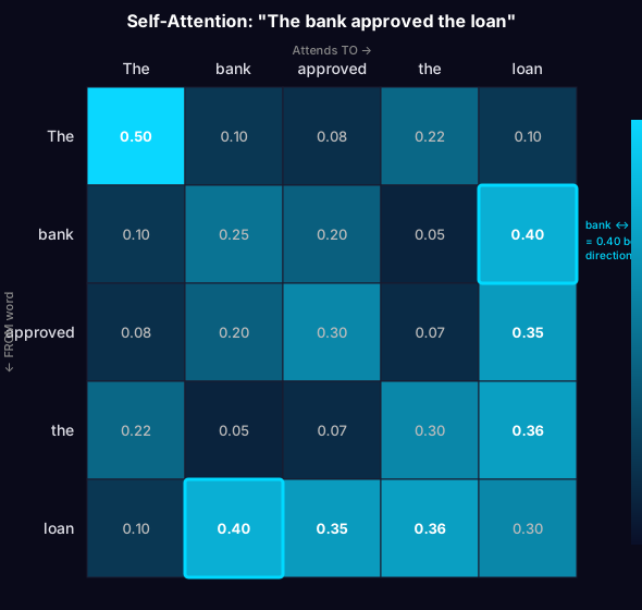
Each row = a word's attention distribution. Notice bank ↔ loan = 0.40 in both directions (symmetric). “The” attends mostly to itself (0.50).

Encoder vs. Decoder — The Big Picture

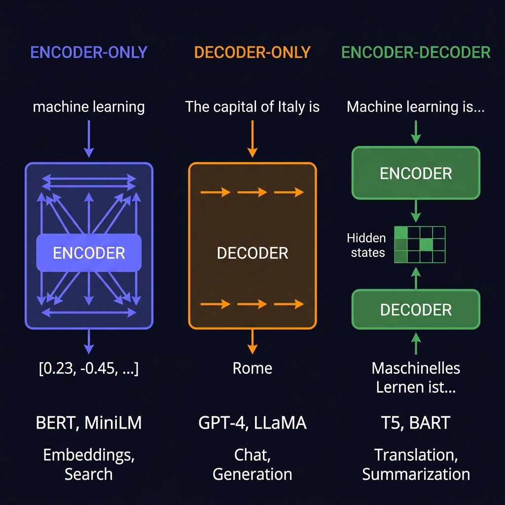
Three architecture families: different attention patterns, different capabilities, different use cases.

Encoder vs. Decoder — Details

ENCODER-ONLY

"machine learning"

⬇️

🔲 ENCODER
Bidirectional — sees all tokens

⬇️

                    [0.23, -0.45, ...] 384 dims
                

BERT · MiniLM · RoBERTa

Best for: embeddings, search, classification

DECODER-ONLY

"The capital of Italy is"

⬇️

🔲 DECODER
Causal — sees only past tokens

⬇️

"The capital of Italy is Rome"

GPT-4 · LLaMA · Mistral

Best for: chat, generation, code

ENCODER-DECODER

"Machine learning is..."

⬇️

🔲 ENCODER → hidden states

⬇️

🔲 DECODER → uses hidden states

⬇️

"Maschinelles Lernen ist..."

T5 · BART · mBART

Best for: translation, summarization

Most modern LLMs are decoder-only — they predict the next token. For embeddings, we use encoder-only models.

How LLMs Actually Work

Input: "The capital of Italy is"

→ probability distribution:

Rome	87.3%
Milan	4.1%
Roma	3.8%
the	1.2%
...	3.6%

The Generation Loop

1. Tokenize input
2. Process through transformer layers
3. Compute probabilities for next token
4. Sample → "Rome"
5. Append to input → repeat from step 2

This is called autoregressive generation — one token at a time, each conditioned on all previous tokens.

An LLM is a next-token predictor. It doesn't know facts — it predicts what text is likely to come next, based on patterns in training data.

The Training Objective — What Is the Model Actually Learning?

During training, the model optimizes a single objective: predict the next token.

L(θ) = − Σ_t=1^T log P(x_t | x₁, ..., x_t-1; θ)

What each part means

θ = all model parameters (weights)
x_t = the actual next token in the training data
P(x_t|...) = model's predicted probability for that token
log = penalizes wrong predictions more than it rewards correct ones
-Σ = sum over ALL positions, minimize total loss

The surprising consequence

The model ONLY learns "what comes next"
Everything else is emergent:
Following instructions → emergent
Writing code → emergent
Translating languages → emergent
Reasoning → emergent

A model trained on "predict the next word" learns grammar, facts, reasoning, and code — all as byproducts of next-token prediction.

🚨 Hallucination

Because LLMs predict plausible text — not truthful text — they can confidently generate false information.

Real Examples of Hallucination

📚 Citing academic papers that don't exist
💻 Importing Python libraries that were never written
📊 Stating revenue figures that are completely fabricated
⚖️ A US lawyer submitted AI-generated brief with 6 fake case citations (2023)

❌ Why It Happens

The model doesn't know facts — it predicts likely-sounding text. If the training data is sparse, it fills gaps with plausible fiction.

✅ How to Mitigate

RAG (Lecture 3) — ground answers in real documents
Temperature = 0 — reduce randomness
Fact-checking — always verify critical outputs

Never deploy an LLM without a way to verify its outputs. This is why we build RAG systems in this course.

Temperature: What It Really Does

Temperature divides the logits before softmax. It changes how “sharp” or “flat” the probability distribution is.

P(token_i) = softmax(logit_i / T) = e^logit_i/T / ∑ e^logit_j/T

Prompt: “The capital of France is” — model outputs raw logits: Paris = 5.0, Lyon = 2.0, Berlin = 1.0

	Logit / T	“Paris”	“Lyon”	“Berlin”	Effect
❄️ T = 0.2	logit / 0.2	99.4%	0.5%	0.1%	Very sharp — always Paris
🎯 T = 1.0	logit / 1.0	84.4%	10.6%	5.0%	Balanced
🌋 T = 2.0	logit / 2.0	49.0%	27.2%	23.8%	Flat — anything could happen

Low T: divides by a small number → logits become larger → softmax becomes sharper → top token wins

High T: divides by a big number → logits become smaller → softmax becomes flatter → any token can win

Temperature does NOT change the model's knowledge. It only changes how we sample from the same distribution. But how does sampling actually work?

How Sampling Works — The Weighted Dice

The model does NOT always pick the highest probability. It rolls a weighted dice.

Probabilities after softmax:

Paris 50% Lyon 30% Berlin 20%

↑ Spinning wheel — each word gets a slice proportional to its probability

The model spins the wheel. Most spins land on Paris (50%), but sometimes Lyon (30%) or Berlin (20%).

T = 0 is special:

No dice, no spinning. Just pick the highest logit, always. Same prompt = same answer, 100% reproducible.

Why Different Answers Each Time?

You send “The capital of France is” 3 times at T = 0.7:

Run 1: dice lands on → “Paris”

Run 2: dice lands on → “Lyon”

Run 3: dice lands on → “Paris”

The probabilities never changed. The random spin gave different results.

Equal Probability?

3 tokens at 33.3% each? → perfectly fair dice. Pure randomness.

Why Not Just Pick the Highest?

“Italy is known for its history. It is also known for its culture. It is also known for its food. It is also known for...”

↑ Greedy decoding — always top token → gets stuck in loops! Sampling adds variety = natural, human-like text.

Every token generation is a dice roll. T = 0 = no dice (deterministic, but can loop). T = 0.7 = natural variety. T = 1.5+ = wild surprises.

Temperature in Practice

Same model, same prompt — only temperature changes the output.

Prompt: “Write a one-sentence summary of machine learning.”

❄️ T = 0 — Deterministic

“Machine learning is a subset of artificial intelligence that enables computers to learn from data without being explicitly programmed.”

Always the same output. Best for: data extraction, classification, factual Q&A

🎯 T = 0.7 — Balanced

“Machine learning allows computers to discover patterns in data and improve their performance over time, much like how humans learn from experience.”

Creative but coherent. Best for: writing, brainstorming, chat. Most common setting.

🌋 T = 1.5 — Wild

“Machine learning unfolds as a computational symphony where algorithms dance through probabilistic landscapes to sculpt emergent understanding.”

Surprising but can be incoherent. Rarely used in production.

❄️ 0 ──── 0.7 ──── 1.0 ──── 1.5+ 🌋

precise, repeatable ←→ creative, surprising

Scale Makes the Difference

Model	Parameters	Training Data
BERT (2018)	340M	16 GB
GPT-3 (2020)	175B	570 GB
LLaMA 3 (2024)	405B	15T tokens
GPT-4 (2023)	~1.8T*	~13T tokens

*estimated

Emergent Abilities

At ~10B params: Chain-of-thought reasoning
At ~100B params: Code generation, translation
At ~1T params: Complex multi-step reasoning

Perplexity — How We Measure LLMs

The standard metric: "on average, how many tokens is the model choosing between?"

PPL = exp(−1/N · Σ_t log P(x_t | x_<t))

Model	Perplexity ↓
GPT-2 1.5B (2019)	~35
GPT-3 175B (2020)	~20
LLaMA 7B (2023)	~7
LLaMA 65B (2023)	~4

Approximate, varies by benchmark dataset

Intuition

PPL = 10 → model is ~90% sure of the next token
PPL = 100 → choosing among ~100 options
Lower = better
A random model: PPL ≈ vocab size (~50,000)

📄 Touvron et al., "LLaMA: Open and Efficient Foundation Language Models", Meta 2023

📏 Context Window

The context window is the model's working memory — how much text it can "see" at once.

Model	Context Window	≈ Pages of Text
GPT-3.5	4K tokens	~3 pages
GPT-4	128K tokens	~100 pages
Claude 3.5	200K tokens	~150 pages
Gemini 1.5	1M+ tokens	~750 pages

What happens when you exceed it?

Text gets truncated — the model "forgets" earlier content
"Lost in the middle" — models pay more attention to the start and end of context, less to the middle
Larger windows = more expensive (more tokens to process)
This is WHY we need RAG (Lecture 3) — to fit only relevant info into the window

From Pre-Training to Prompting

Three levels of effort — from building a model to just talking to it:

1. Pre-Training

Months $2M–$100M+

Train from scratch on massive internet data. Only done by Google, Meta, OpenAI, etc.

⬇️ adapt to your domain

2. Fine-Tuning

Hours–Days $10–$1,000

Adapt a pre-trained model with your data → Lectures 8–9

⬇️ or skip training entirely

3. Prompting

Seconds $0.001

Zero training — just write clever instructions → Lecture 2

Most enterprise use cases start with prompting (cheapest, fastest), add RAG for accuracy, and only fine-tune when needed. You almost never pre-train from scratch.

RLHF — How Models Learn to Follow Instructions

Pre-training alone produces a text completer, not an assistant. RLHF bridges the gap.

Step 1: Pre-training — predict next token on internet text

Result: knows language, facts, patterns. But not helpful yet.

↓

Step 2: SFT — train on human-written Q&A pairs

Result: can answer questions. But sometimes verbose or unhelpful.

↓

Step 3: RLHF — humans rank outputs, train reward model, optimize via PPO

Result: helpful, harmless, honest. This is ChatGPT.

L_RLHF = −E[r(x, y)] + β · KL[π_θ || π_ref]

Maximize reward while staying close to original model via KL divergence penalty

📄 Ouyang et al., "Training language models to follow instructions with human feedback", NeurIPS 2022

Next Lecture

Lecture 2 will cover:

Tokenization — BPE algorithm, why Italian costs more
Embeddings — Word2Vec, cosine similarity, vector spaces
Multilingual models — cross-lingual alignment
🔬 Hands-on Lab — semantic search exploration

❓

Questions?

Thank you!

Kamyar Zeinalipour — Zucchetti LLM Course

The TransformerBlueprint

Today’s Agenda

The TransformerBlueprint

What is an LLM, Really?

What it IS

What it is NOT

Before Transformers

RNNs / LSTMs

Transformers (2017)

The Timeline: How We Got Here

The Papers That Built Modern AI

The Transformer Architecture

Why Position Matters

Positional Encoding — The Math

Why sin/cos?

Modern alternative: RoPE

Self-Attention: The Core Idea

📚 Library Analogy for Q, K, V

Self-Attention: Step-by-Step with Numbers

The 6 Steps

What Just Happened?

Multi-Head Attention — The Full Picture

Inside One Transformer Block

How Q, K, V Are Created

Concrete Trace: “bank”

Attention in Action

Encoder vs. Decoder — The Big Picture

Encoder vs. Decoder — Details

How LLMs Actually Work

The Generation Loop

The Training Objective — What Is the Model Actually Learning?

What each part means

The surprising consequence

🚨 Hallucination

Real Examples of Hallucination

❌ Why It Happens

✅ How to Mitigate

Temperature: What It Really Does

How Sampling Works — The Weighted Dice

Why Different Answers Each Time?

Equal Probability?

Why Not Just Pick the Highest?

Temperature in Practice

Scale Makes the Difference

Emergent Abilities

Perplexity — How We Measure LLMs

Intuition

📏 Context Window

What happens when you exceed it?

From Pre-Training to Prompting

RLHF — How Models Learn to Follow Instructions

Next Lecture

Questions?

The Transformer
Blueprint

The Transformer
Blueprint