Zucchetti LLM Course — Lecture 9

Efficient
Fine-Tuning

LoRA • QLoRA • From Theory to Production

Teaching models new behaviors — without breaking the bank

Kamyar Zeinalipour

Today’s Agenda

2 hours full theory • 10 min break

S0 — Understanding Fine-Tuning — Where We Are & What It Means

S1 — When to Fine-Tune — Decision Flowchart & Real-World Cases

S2 — LoRA & QLoRA — The Core Mechanics + Worked Example

S3 — The Training Kitchen — Practical Tricks + Evaluation

S4 — From Data to Production — Case Study & Common Mistakes

☕ Break — 10 minutes

S5 — Beyond SFT — DPO & Alignment

💻 S6 — SFT in Practice — Code Walkthrough: Normal SFT vs Thinking SFT

Section 0

Understanding Fine-Tuning

Where we are, what it means, and how training works

The Story So Far

Eight lectures of working AROUND the model — today we work ON it

L1 — Transformer Architecture — how the model works inside

L2–L3 — Tokenization, Embeddings, Prompting — talk to the model

L4–L6 — RAG, Advanced RAG, Graph RAG — give it external knowledge

L7 — Agentic RAG — give it tools

L8 — Evaluation — measure everything

L9 — Fine-Tuning — change the model itself ⬅ TODAY

In L1–L8 we worked around the model: better prompts, external knowledge, tools, evaluation. Today we go inside — we change the weights themselves.

External vs Internal Approaches

Two fundamentally different strategies for improving an LLM

🌍 External (L2–L8)

Prompting — changes the INPUT

RAG — adds knowledge AT RUNTIME

Agents — adds tools AT RUNTIME

The model weights never change. Every improvement happens outside.

🧬 Internal (Today)

Fine-tuning — changes the MODEL WEIGHTS

Behavior becomes permanent

No retrieval needed, no prompt tricks

The model itself is different after training.

External = giving someone a phrasebook and a calculator. Internal = teaching them the language and the math.

What IS Fine-Tuning?

Continue training a pre-trained model on YOUR data

Pre-trained Model
Someone else trained this
on trillions of tokens

→

Your Data
500–5000 examples
of desired behavior

→

Fine-tuned Model
Same knowledge
new behavior

Key Concepts

Pre-training — the expensive part. Done by Meta, Alibaba, Google. Costs millions of dollars. Teaches language, facts, reasoning. You don’t do this.

Fine-tuning (SFT) — the cheap part. Done by YOU. Costs minutes to hours. Teaches your specific task, format, and style.

Full Fine-Tuning

Update ALL weights
Maximum quality, maximum cost

Efficient Fine-Tuning (LoRA)

Update 0.25% of weights
Today’s main focus

The Training Loop

How a model learns from data — the engine behind all fine-tuning

① Forward
Feed input
get prediction

→

② Loss
How wrong
is the output?

→

③ Backward
Compute gradients
who caused the error?

→

④ Update
Adjust weights
reduce the error

The Loss Function

$\mathcal{L} = -\log P(\text{correct token} \mid \text{previous tokens})$

Same next-token prediction from Lecture 1. The model sees your training example and tries to predict each token. The loss measures how far off it was. Gradients tell the optimizer which weights to adjust.

🔄 Repeat

Do this for every example in your dataset. One full pass = 1 epoch. Typically 1–3 epochs for fine-tuning. After each batch, the model gets slightly better at your task.

L1 callback: the attention mechanism, Q/K/V projections — those are the weights being updated in this loop. With LoRA, we’ll update only tiny adapters attached to them.

Full SFT: The Straightforward Approach

Update ALL parameters — simple, effective, but expensive

What Happens During Full SFT

Every single weight in the model — all 494 million in Qwen2.5-0.5B, or all 7 billion in Llama-3 — gets updated via gradient descent. Nothing is frozen.

from transformers import AutoModelForCausalLM
from trl import SFTTrainer, SFTConfig

# Load model — ALL parameters are trainable
model = AutoModelForCausalLM.from_pretrained("Qwen/Qwen2.5-0.5B-Instruct")

# Train — updates ALL 494M parameters
trainer = SFTTrainer(model=model, train_dataset=data,
    args=SFTConfig(output_dir="./output", num_train_epochs=2))
trainer.train()  # Every weight changes

✅

Pros

Highest possible quality
Maximum flexibility
Well-understood technique

⚠

But...

Needs 40–80+ GB VRAM
Risk of catastrophic forgetting
Creates a full model copy per task

Full SFT works perfectly. The results are excellent. So what’s the problem? → Let’s talk about cost...

Section 1

When to Fine-Tune

Decision framework: prompting vs RAG vs fine-tuning

The Decision Matrix Revisited From L4

In L4 we learned when to fine-tune — now we learn how

Criterion	Prompting	RAG	Fine-Tuning
Setup cost	Minutes	Hours	Hours
New knowledge	No	Yes	Limited
Behavior change	Some	No	Yes
Output style	Fragile	Inherited	Consistent
Latency	Fast	Slower	Fast

Fine-tuning wins when you need consistent behavior, style, or format — not when you need new knowledge (that’s RAG).

What Fine-Tuning Actually Is

Not teaching knowledge — teaching behavior

❌ Common Misconception

“Fine-tuning teaches the model new facts”

Want to add company knowledge? Use RAG.

✅ What It Really Does

“Fine-tuning teaches the model a new accent”

Output format, tone, domain vocabulary, task behavior

Concrete Example — Zucchetti Medical Ticket Classifier

Before fine-tuning: “This seems urgent because the patient mentioned chest pain…”

After fine-tuning: {"priority": "P1", "category": "CARDIAC", "escalate": true}

Same knowledge, completely different behavior and output format.

Think of it like this: Knowledge = books in a library (RAG adds more books). Fine-tuning = teaching someone a new accent — they use the same words, but speak differently.

The Decision Flowchart

When to fine-tune, RAG, or prompt — a practical guide

🤔 Do you need the model to know NEW FACTS?

YES

Use RAG

Vector DB + retrieval.
Model cites your documents.

↓

🎯 Do you need CONSISTENT behavior, format, or style?

YES

Fine-Tune

LoRA/QLoRA on 500+ examples.
Bakes behavior into the model.

NO / One-off

Prompt Engineering

System message + few-shot.
Fast, flexible, no training.

Most teams should try prompting first, then RAG, then fine-tuning. Fine-tuning is the last step, not the first.

Real-World Fine-Tuning Success Stories

Different domains, different scales — same idea: teach the model new behavior

🏥

Medical Ticket Classifier

Task: Triage patient tickets into P1–P5 with structured JSON

Data: 800 labeled tickets

Before: 65% format compliance

After: 98% compliance

Efficient fine-tuning, 2 epochs, 25 min

💻

Code Review Assistant

Task: Generate code reviews in company style

Data: 2,000 past reviews

Before: Generic feedback

After: Team-specific style

Efficient fine-tuning, 3 epochs, 45 min

🌍

Multilingual Support

Task: Customer service in IT/DE/FR

Data: 1,500 conversations per language

Before: English-centric responses

After: Native-quality replies

Separate adapter per language (~5 MB each)

🧬 When Full SFT Shines: Domain-Changing Tasks

Some tasks completely change what the model does — here, updating ALL weights is worth the cost:

🧪 Protein Generation
ProGen, ESMFold — transformers trained on amino acid sequences to design novel proteins

💊 Drug Discovery
MolGPT, ChemBERTa — transformers fine-tuned on SMILES molecular strings

🧬 DNA / Genomics
DNABERT, Nucleotide Transformer — trained on DNA base-pair sequences (A, T, G, C as tokens)

Behavior tuning (tickets, reviews, chat) → efficient fine-tuning is enough. Domain change (proteins, molecules) → Full SFT may be necessary.

The Problem with Full SFT

It works — but at what cost?

💰

Expensive

7B model = 40–80+ GB VRAM
70B = multiple A100s
~$15,000/GPU

⏰

Slow

Hours of GPU time
for meaningful training
vs. minutes with LoRA

🧠

Catastrophic Forgetting

Overwrite useful
pre-trained knowledge
Model “forgets” how to chat

Why So Much VRAM?

$\text{VRAM} \approx \text{params} \times \text{bytes per param} \times \text{overhead}$

7B params × 2 bytes (fp16) = 14 GB just for weights. Add gradients (14 GB) + Adam optimizer states (56 GB in fp32: momentum + variance) = 84+ GB for full SFT. With mixed precision tricks: ~28–40 GB. LoRA only stores gradients for the tiny adapters.

What if we could train 0.25% of the parameters and get 95% of the quality?

Full SFT is like repainting your entire house to change the color of one room. LoRA is like repainting just that room.

Section 2

LoRA & QLoRA

The low-rank trick that changed everything

The Low-Rank Hypothesis ICLR 2022

Most weight updates during fine-tuning live in a low-dimensional subspace

The Insight

A weight matrix $W$ has dimensions $d \times k$ (e.g., 4096 × 4096 = 16.7M params).

But the useful update $\Delta W$ has much lower rank — rank 8–32 captures most of the signal.

$W_{\text{new}} = \underbrace{W_{\text{frozen}}}_{\text{do not touch}} + \underbrace{\frac{\alpha}{r} \cdot B \cdot A}_{\text{train this}}$

Initialization Trick

$A$ is initialized with random Gaussian, $B$ is initialized with zeros. So at the start: $\Delta W = B \cdot A = 0$. The model starts exactly as the base model and gradually learns the adaptation.

Matrix A

$d \times r$ (4096 × 8)

= 32,768 params

Matrix B

$r \times k$ (8 × 4096)

= 32,768 params

Instead of updating 16.7M parameters per layer, we train just 65K. That’s a 256× reduction.

Hu et al. (2022) — “LoRA: Low-Rank Adaptation of Large Language Models” — ICLR 2022

LoRA — The Intuition

Why does low-rank work? A visual explanation.

Analogy: The GPS Correction

The base model’s weight matrix is a detailed map of the world. Fine-tuning for medical text? You don’t redraw the entire map — you just add a small overlay for the hospital district.

That overlay is low-rank — it only changes a few “directions” in weight space.

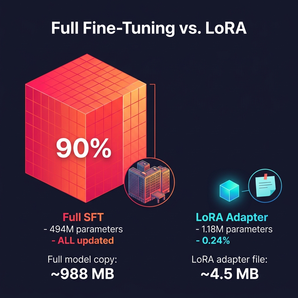
Qwen2.5-0.5B Numbers

Metric	Full SFT	LoRA (r=8)
Trainable	494M (100%)	1.18M (0.24%)
Storage	~988 MB	~4.5 MB

LoRA adapters are tiny files (~5 MB) that sit on top of a frozen base model. You can have dozens of adapters for different tasks, all sharing the same base.

LoRA — Worked Example

Let’s trace through one attention layer step by step

Setup: One Q-projection Layer

Model: Qwen2.5-0.5B • Hidden dimension: $d = 896$ • LoRA rank: $r = 16$

Component	Shape	Parameters	Storage
$W_{q}$ (frozen)	896 × 896	802,816	❄ not trained
$A$ (down-project)	896 × 16	14,336	~57 KB
$B$ (up-project)	16 × 896	14,336	~57 KB
Total adapter	—	28,672	~114 KB

Compression: $\frac{802{,}816}{28{,}672} \approx$ 28× fewer parameters per layer

With 24 attention layers, each with Q, K, V, O projections, total LoRA params = 28,672 × 4 × 24 = ~2.75M trainable (vs 494M total = 0.56%).

Inside the Transformer: Where LoRA Lives

Which layers get adapters? From L1

🧠 Attention Block

🔥 q_proj — query projection LoRA

🔥 k_proj — key projection LoRA

🔥 v_proj — value projection LoRA

🔥 o_proj — output projection LoRA

All 4 attention projections — this is the minimum recommended set.

⚙ MLP Block

❄ gate_proj — gating Optional

❄ up_proj — expansion Optional

❄ down_proj — compression Optional

Adding MLP layers increases params but can help for complex tasks.

Practical Recommendation

Start with attention only (q, k, v, o). If quality isn’t sufficient, add MLP layers. The original LoRA paper only used q and v — modern practice targets all attention.

L1 callback: these are the same Q, K, V matrices from the self-attention mechanism we learned in Lecture 1. LoRA injects small adapters into each one.

LoRA Mechanics — Step by Step

Freeze everything, train tiny adapters

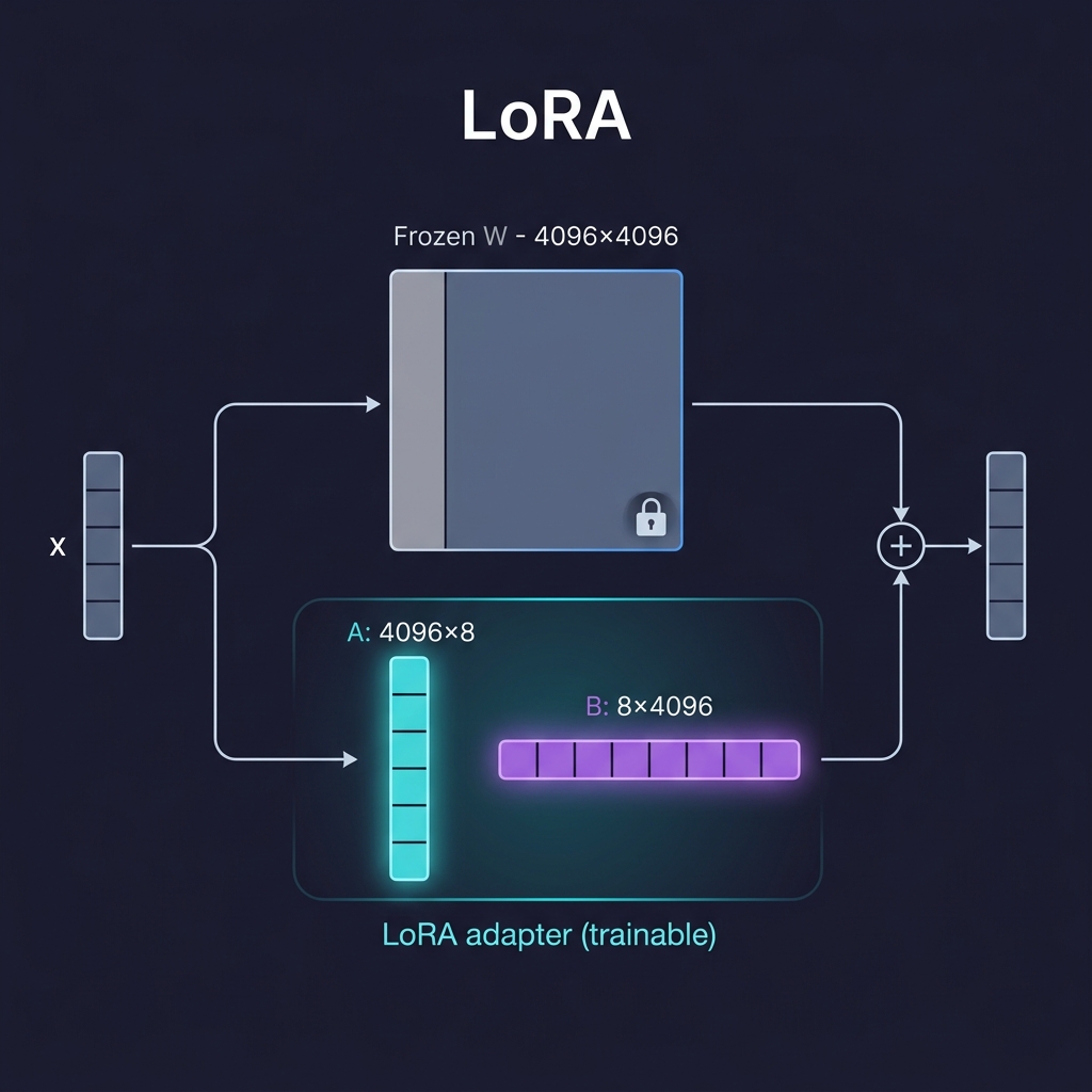
Forward Pass

$h = W_{frozen} \cdot x + \frac{\alpha}{r} \cdot B \cdot A \cdot x$

❄ Path 1: Frozen W × x — never changes

🔥 Path 2: α/r × B × A × x — trainable adapter

Output = sum of both paths

Three Design Choices

Parameter	Controls	Typical
`r` (rank)	Adapter size	8, 16, 32
`lora_alpha`	Scaling factor	$2 \times r$ or $r$
`target_modules`	Which layers	q, k, v, o

L1 callback: the Q, K, V projections from the transformer attention — those are the target_modules we inject LoRA into

Choosing LoRA Hyperparameters

Practical guidelines — don’t overthink it

The Scaling Formula

$\text{Effective update} = \frac{\alpha}{r} \times B \cdot A \cdot x$

If $\alpha = 16$ and $r = 8$: scaling = $\frac{16}{8} = 2.0$. If $\alpha = r$: scaling = $1.0$.

Higher scaling = adapter has more influence. Lower scaling = gentler adaptation.

Scenario	Rank (r)	Alpha	Target Modules	Example
Light style change	8	16	q_proj, v_proj	Always reply in Italian
Domain adaptation	16–32	32–64	All attention + MLP	Medical ticket classifier
Complex behavior	64+	128+	All linear layers	Code generation specialist

Start with r=16, alpha=32, all attention layers. Increase rank only if performance plateaus. More data beats higher rank every time.

QLoRA: Fine-Tuning on a Laptop NeurIPS 2023

4-bit quantization + LoRA = train a 7B model in 6 GB

Key Innovation: NormalFloat4 (NF4)

Quantize the frozen base model to 4-bit. LoRA adapters stay in float16. During training: dequantize → forward → backward on adapters only.

What Does 4-bit Mean?

$\text{Memory} = \frac{\text{params} \times \text{bits}}{8 \times 10^9} \text{ GB}$

fp16 (16-bit): $\frac{7 \times 10^9 \times 16}{8 \times 10^9} = $ 14 GB • NF4 (4-bit): $\frac{7 \times 10^9 \times 4}{8 \times 10^9} = $ 3.5 GB

The LoRA adapters (~50 MB) run at full float16 precision on top of the 4-bit base.

Full SFT
40–80+ GB

→

LoRA
12–16 GB

→

QLoRA
6–8 GB

Dettmers et al. (2023) — “QLoRA: Efficient Finetuning of Quantized LLMs” — NeurIPS 2023

Full SFT vs LoRA vs QLoRA

Choosing the right method for your constraints

Method	VRAM (7B)	Training Time	Quality	Cost
Full SFT	40–80+ GB	Hours	Highest	$$$
LoRA	12–16 GB	30–60 min	High	$$
QLoRA	6–8 GB	45–90 min	Good–High	$

🚀 Unsloth Framework

Hand-written CUDA kernels: 2× faster training, 60% less memory. Fully compatible with HuggingFace. Free and open-source.

QLoRA + Unsloth is the sweet spot for most teams. Train a 7B model on a single consumer GPU (RTX 3090 / 4090).

LoRA in 5 Lines of Code

From theory to practice — it’s really this simple

from peft import LoraConfig, get_peft_model

# 1. Define the adapter configuration
config = LoraConfig(
    r=16,                                          # Rank
    lora_alpha=32,                                 # Scaling (alpha/r = 2.0)
    target_modules=["q_proj", "k_proj",            # Which layers
                    "v_proj", "o_proj"],
    lora_dropout=0.05,                             # Regularization
    task_type="CAUSAL_LM",                         # Language model
)

# 2. Wrap the frozen model with LoRA adapters
model = get_peft_model(base_model, config)

# 3. Check: how many parameters are trainable?
model.print_trainable_parameters()
# trainable params: 1,572,864 || all params: 495,606,784 || 0.32%

That’s it. Two lines to configure, one line to apply. The get_peft_model() call freezes all original weights and injects the tiny LoRA matrices. We’ll see the full training loop in Section 6.

Before vs After Fine-Tuning

Same model, same question — dramatically different behavior

💬 Question: “A 45-year-old male presents with crushing chest pain radiating to his left arm. ST-elevation in V1–V4. What is the diagnosis?”

❌ Base Model (Before)

“This is a complex medical case that requires careful analysis. The patient’s symptoms could indicate several conditions including myocardial infarction, angina pectoris, or possibly a pulmonary embolism. It would be important to consider the full clinical picture and conduct further diagnostic tests such as blood work and imaging studies…”

⚠ Vague, hedging, no structured output, verbose

✅ LoRA Fine-Tuned (After)

“Diagnosis: Acute ST-elevation myocardial infarction (STEMI).
Urgency: P1 — Immediate.
Key findings: Crushing chest pain + left arm radiation + ST-elevation V1–V4.
Action: Activate cath lab, administer aspirin 325mg.”

✅ Structured, decisive, actionable, domain-specific format

Same 0.5B model, same knowledge. The fine-tuned version learned a new behavior: structured medical triage format. This is what 800 training examples and 25 minutes of LoRA training achieves.

Section 3

The Training Kitchen

Practical tricks that make or break your fine-tune

Gradient Accumulation

Simulate large batches on small GPUs

The Problem

Your GPU fits only batch_size=2, but stable training needs an effective batch of 16.

The Solution

Run 8 forward+backward passes, accumulate the gradients, then do one optimizer step.

$\text{effective\_batch} = \underbrace{\text{per\_device\_batch}}_{\text{what fits in GPU}} \times \underbrace{\text{grad\_accum\_steps}}_{\text{accumulate}} \times \text{num\_GPUs}$

Example: 2 × 8 × 1 = 16 effective batch size

TrainingArguments(
    per_device_train_batch_size=2,     # What fits in GPU memory
    gradient_accumulation_steps=8,      # Accumulate 8 micro-batches
    # → effective_batch_size = 2 × 8 = 16
)

Rule: maximize real batch size first (less noise), then use accumulation for the rest. Avoid batch_size=1 with high accumulation — it can degrade quality.

Sequence Packing Efficiency Boost

Stop wasting tokens on padding

❌ Without Packing

[seq1····][PAD][PAD][PAD][PAD]
[seq2··][PAD][PAD][PAD][PAD][PAD]
[seq3·······][PAD][PAD][PAD]

~60% of tokens are padding = wasted compute

✅ With Packing

[seq1][EOS][seq2][EOS][seq3·]
[seq4··][EOS][seq5][EOS][seq6]
[seq7····][EOS][seq8][PAD]

Sequences concatenated, separated by EOS

SFTTrainer(
    ...,
    packing=True,           # Enable sequence packing
    max_seq_length=2048,    # Pack into 2048-token blocks
)

Without packing = every passenger gets their own bus (mostly empty seats). With packing = fill every seat before sending the next bus.

Chat Templates Critical

The format must match between training and inference

ChatML Format (Industry Standard)

<|im_start|>system
You are a medical assistant.<|im_end|>
<|im_start|>user
What is the dosage for amoxicillin?<|im_end|>
<|im_start|>assistant
The standard dosage is 500mg every 8 hours.<|im_end|>

❌ Wrong Template

Train with ChatML, infer with Llama format → model outputs gibberish

✅ Correct Way

# Always use the tokenizer's
# built-in template:
tokenizer.apply_chat_template(
    messages, tokenize=True
)

Golden rule: never manually format chat strings. Always use tokenizer.apply_chat_template() — it reads the model’s native format automatically.

Loss Masking / Completion-Only Training

Train on answers only — don’t waste capacity predicting prompts

The Problem

Without masking, the model tries to predict every token — including the prompt it was given as input. That’s like practicing for a test by memorizing the questions instead of the answers.

The Solution: Mask Prompt Tokens

[system] You are a medical assistant [user] What is amoxicillin?
Labels: [-100] [-100] [-100] ... [-100] ← ignored
[assistant] Amoxicillin is a penicillin-type antibiotic used to...
Labels: [token_ids...] ← loss computed here only

from trl import DataCollatorForCompletionOnlyLM
collator = DataCollatorForCompletionOnlyLM(
    response_template="<|im_start|>assistant\n",  # Mask everything before this
    tokenizer=tokenizer,
)

Loss masking focuses 100% of learning on generating good answers. Without it, 50%+ of gradient updates are wasted on predicting prompts.

NEFTune — Free Accuracy Boost ICLR 2024

One line of code, measurable improvement

How It Works

During training, add random noise to the embedding vectors. This prevents the model from memorizing exact training examples. Like adding a slight blur to training images in computer vision.

$\tilde{e} = e + \frac{\alpha}{\sqrt{L \cdot d}} \cdot U(-1, 1)$

When to Use

Small datasets (<1000 examples)
Signs of overfitting
Instruction tuning tasks

Settings

Start with alpha=5
Sweep: {3, 5, 10}
No other config changes needed

SFTTrainer(..., neftune_noise_alpha=5)  # That's literally it!

Jain et al. (2024) — “NEFTune: Noisy Embeddings Improve Instruction Finetuning” — ICLR 2024

Flash Attention & Gradient Checkpointing

Two memory-saving techniques every fine-tuner should know

⚡ Flash Attention 2

What: Optimized tiled GPU computation for the attention mechanism (from L1)

Effect: 2–4× faster attention, 20–40% less end-to-end memory

When: Always enable if hardware supports it

model = AutoModelForCausalLM
  .from_pretrained(
    model_id,
    attn_implementation=
      "flash_attention_2"
)

💾 Gradient Checkpointing

What: Discard activations during forward pass, recompute during backward

Effect: ~30% less memory, ~20% slower

When: Last resort for OOM errors

TrainingArguments(
    ...,
    gradient_checkpointing=True,
)

Flash Attention = free speed. Gradient Checkpointing = last resort for OOM. Stack both with QLoRA for maximum efficiency.

The Complete Training Checklist ✅

Your reference card — bookmark this slide

Setting	Recommendation	Why
Learning rate	`2e-4`	Standard for LoRA/QLoRA
Optimizer	`adamw_torch` or `paged_adamw_8bit`	Paged = less VRAM
Epochs	1–3	More = overfitting risk
Warmup	5–10% of steps	Stabilizes early training
Packing	✅ Enable	Up to 2–3× speed boost
Loss masking	✅ Completion-only	Focus on answers
NEFTune	✅ alpha=5	Free regularization
Flash Attention	✅ If supported	Free speed
Grad. Checkpoint	⚠️ If OOM	Memory vs speed trade-off

Overfitting — The #1 Enemy Warning

Small dataset + too many epochs = memorization, not learning

🚨 Signs of Overfitting

Training loss keeps dropping
But eval loss starts rising
Model outputs exact training examples
Poor performance on unseen inputs

🛡️ Defenses

Early stopping — monitor eval loss
NEFTune — noise regularization
Lower rank — less model capacity
More data — always the best fix
Fewer epochs — often 1–2 is enough

Overfitting is like a student who memorizes the answer key instead of understanding the subject. They ace the practice test but fail the real exam.

Evaluating Your Fine-Tune From L8

The same evaluation framework from L8 — applied to fine-tuning

The Three Checks

Check	What You Measure	How
1. Task Quality	Does the model do the task correctly?	Golden dataset + task-specific metrics (accuracy, F1)
2. Format Compliance	Does it output the right format?	Parse outputs, check JSON validity, schema match
3. Regression	Did we break general abilities?	Run base model benchmarks (MMLU, HellaSwag) before/after

📉 Training Metrics

Watch during training:
Training loss (should decrease)
Eval loss (should NOT increase)
If eval loss rises = overfitting

🔍 Post-Training Eval

Run after training:
Hold-out test set (20% of data)
Before/after comparison table
LLM-as-Judge (from L8)

L8 callback: the golden dataset + LLM-as-Judge technique works for fine-tuning evaluation too. Same metrics (faithfulness, relevance), different context.

Framework Comparison

Choose your tool — all produce compatible LoRA adapters

Framework	Speed	Memory	Ease of Use	Best For
HuggingFace PEFT + TRL	Baseline	Baseline	Excellent	Flexibility, research
Unsloth	2× faster	60% less	Easy	Production speed
LlamaFactory	Good	Good	YAML config	Beginners, no-code
Axolotl	Fast	Good	Config-heavy	Advanced multi-task

Key Point: No Lock-In

All frameworks produce standard PEFT adapters. Train with Unsloth → deploy with HuggingFace. Train with LlamaFactory → merge with PEFT. The adapter format is universal.

Section 4

From Data to Production

Datasets, merging, and deployment

Instruction Dataset Formats

Two main formats — pick one and be consistent

Alpaca Format (Single-Turn)

{
  "instruction": "Classify this 
    medical ticket",
  "input": "Patient reports severe
    chest pain after exercise",
  "output": "Priority: P1\n
    Category: CARDIAC\n
    Action: IMMEDIATE_ESCALATION"
}

Conversation Format (Multi-Turn)

{
  "messages": [
    {"role": "system",
     "content": "You classify 
      medical tickets."},
    {"role": "user",
     "content": "Chest pain..."},
    {"role": "assistant",
     "content": "{\"priority\":\"P1\"}"}
  ]
}

Format consistency matters more than dataset size. One badly formatted example causes more damage than 100 good ones fix.

How Much Data Do You Need?

Less than you think — if it’s high quality

Dataset Size	What You Can Achieve	Zucchetti Example
50–100	Style/format changes	Always output structured JSON
500–2,000	Domain-specific tasks	Medical ticket classification
2,000–5,000	Complex behavior	Multi-step clinical extraction
5,000+	Approaching full SFT quality	General medical assistant

Data Quality Checklist ✅

Consistent formatting — every example follows the same template
No contradictions — don’t say “chest pain = P1” in one and “chest pain = P3” in another
Balanced categories — don’t have 90% P3 and 5% P1 tickets
Human-validated — a domain expert reviewed the outputs

500 perfect examples beat 50,000 noisy ones. Spend time curating, not collecting.

Adapter Merging & Multi-Adapter Serving

From trained adapter to production model

Option A: Merge into Base

Permanently bake LoRA weights into the base model.

merged = model.merge_and_unload()
merged.save_pretrained("./merged")

Simpler deployment, no adapter overhead

Option B: Serve Dynamically

One base model, hot-swap LoRA adapters per request.

vLLM and LoRAX support this natively.

Multi-tenant: medical adapter, legal adapter, HR adapter

Advanced Merging: TIES & DARE

When merging multiple LoRA adapters into one model: TIES trims redundant params and resolves sign conflicts. DARE randomly drops 90%+ of params and rescales. Both reduce interference between task-specific adapters.

Export & Deployment Pipeline

The complete path from training to production

🔥 Train
LoRA/QLoRA

→

🔗 Merge
merge_and_unload()

→

📦 Quantize
GGUF / AWQ

→

🚀 Deploy
Ollama / vLLM

Export Format	Use Case	Tools
GGUF	Local deployment (laptops, edge devices)	Ollama, llama.cpp
Safetensors	Cloud deployment, sharing on HuggingFace	transformers, vLLM
AWQ / GPTQ	GPU-optimized quantized serving	vLLM, TGI

The pipeline is like cooking: Train = cook the meal. Merge = plate it. Quantize = portion control. Deploy = serve to customers.

Case Study: End-to-End Fine-Tuning Project

From zero to production — realistic timeline

📊 Data
2–3 hours

→

🧹 Clean
1–2 hours

→

🔥 Train
30 min

→

🔍 Eval
1–2 hours

→

🚀 Deploy
2–4 hours

Key Metrics (Medical Ticket Classifier)

Metric	Prompting Only	After LoRA
Format compliance (valid JSON)	65%	98%
Priority accuracy	72%	94%
Latency (per ticket)	1.2s (RAG lookup)	0.3s (no retrieval)
Monthly cost (1K tickets/day)	~€180	~€45

Notice: training is the FAST part (30 min). Data preparation and evaluation take most of the effort. Total: zero to production in a single day.

Top 5 Fine-Tuning Mistakes Avoid These

Learn from others’ failures

#	Mistake	What Happens	Fix
1	Wrong chat template	Model outputs gibberish at inference	Always use `tokenizer.apply_chat_template()`
2	Not enough data diversity	Model only handles training patterns	Include edge cases, negatives, refusals
3	Training too many epochs	Overfitting — memorizes training data	Start with 1–2 epochs, watch eval loss
4	Skipping evaluation	Ship a broken model to production	Always hold out 20% for testing
5	Contradictory training data	Model gives inconsistent answers	Audit for conflicts before training

Mistake #1 is the most common. If you train with ChatML format but serve with Llama format, every response will be garbage. The tokenizer knows the right format — use it.

☕ Break

10 minutes

When we come back: DPO, alignment, and a full code walkthrough.

Section 5

Beyond SFT

The modern post-training pipeline

The Modern Post-Training Pipeline

How modern open-source models are built

Pre-Training
Trillions of tokens

→

SFT
Teach behavior

→

DPO / RLHF
Align preferences

→

Deploy
Production

SFT = Capabilities

Teach what to do: follow instructions, output JSON, classify tickets, speak in medical terms.

This is what we learned today.

DPO = Preferences

Teach how to choose: prefer helpful over harmful, concise over verbose, accurate over creative.

Refines quality after SFT.

L1 callback: In L1 we learned about RLHF (InstructGPT). DPO is the simpler, modern alternative — no separate reward model needed.

DPO vs RLHF — Quick Overview

Alignment without a reward model

Aspect	RLHF (from L1)	DPO (modern)
Reward model	Required (expensive)	Not needed
Training data	Rankings + reward model	Preference pairs (chosen vs rejected)
Complexity	PPO algorithm, unstable	Simple loss function
Quality	Excellent	Nearly as good

DPO Training Data Example

{
  "prompt": "Explain LoRA in one sentence.",
  "chosen": "LoRA freezes the base model and trains small adapter matrices to 
             efficiently adapt behavior.",
  "rejected": "LoRA is a type of AI thing that makes models better somehow."
}

SFT first, then DPO. SFT teaches the task; DPO refines the quality. You can apply LoRA to both stages.

Rafailov et al. (2023) — “Direct Preference Optimization: Your Language Model is Secretly a Reward Model” — NeurIPS 2023

Section 6

SFT in Practice

Code walkthrough — Normal SFT vs Thinking SFT

The Complete SFT Training Loop

Everything you need — model + LoRA + data + trainer

from transformers import AutoModelForCausalLM, AutoTokenizer
from peft import LoraConfig, get_peft_model
from trl import SFTTrainer, SFTConfig
from datasets import load_dataset

# 1. Load model + tokenizer
model = AutoModelForCausalLM.from_pretrained("Qwen/Qwen2.5-0.5B-Instruct")
tokenizer = AutoTokenizer.from_pretrained("Qwen/Qwen2.5-0.5B-Instruct")

# 2. Apply LoRA
lora_config = LoraConfig(r=16, lora_alpha=32,
    target_modules=["q_proj","k_proj","v_proj","o_proj"],
    task_type="CAUSAL_LM")
model = get_peft_model(model, lora_config)

# 3. Load dataset (we'll see the format next)
data = load_dataset("json", data_files="train.jsonl", split="train")

# 4. Train!
trainer = SFTTrainer(model=model, tokenizer=tokenizer,
    train_dataset=data,
    args=SFTConfig(output_dir="./output", num_train_epochs=2,
        per_device_train_batch_size=4, learning_rate=2e-4,
        logging_steps=10, save_steps=100))
trainer.train()  # That's it!

~25 lines of code to fine-tune any model with LoRA. The magic is in the dataset format — that’s what determines the model’s behavior.

Normal SFT — Dataset Format

Teach the model to follow instructions → give direct answers

📄 Dataset (train.jsonl)

{
  "messages": [
    {"role": "system",
     "content": "You are a medical
      triage assistant. Output JSON."},
    {"role": "user",
     "content": "Patient: chest pain,
      shortness of breath"},
    {"role": "assistant",
     "content": "{\"priority\":\"P1\",
      \"category\":\"CARDIAC\",
      \"action\":\"ESCALATE\"}"}
  ]
}

🤖 Model Learns

Input: system + user message

Output: direct answer in the trained format

Model output:

{"priority":"P1", "category":"CARDIAC", "action":"ESCALATE"}

No reasoning, no explanation — just the answer.

Normal SFT is perfect for: classification, structured output, format compliance, simple Q&A. The model learns to skip thinking and give the answer directly.

Thinking SFT — Dataset Format 2024–2025

Teach the model to reason step-by-step before answering

📄 Dataset with <think> Tags

{
  "messages": [
    {"role": "system", "content": "You are a medical assistant. Think step by step."},
    {"role": "user", "content": "Patient: 45M, crushing chest pain, left arm radiation, ST-elevation V1-V4"},
    {"role": "assistant", "content": "<think>\nStep 1: Crushing chest pain + left arm radiation = classic cardiac presentation.\nStep 2: ST-elevation in V1-V4 = anterior wall involvement.\nStep 3: This pattern = acute STEMI. P1 priority.\nStep 4: Immediate action: cath lab activation.\n</think>\n\n{\"diagnosis\":\"Acute STEMI\", \"priority\":\"P1\", \"action\":\"CATH_LAB\"}"}
  ]
}

🧠 How It Works

The model learns to generate reasoning inside <think>...</think> tags, then produce the final answer. At inference, you can parse and hide the thinking.

💡 Why It Matters

Made famous by DeepSeek-R1 and OpenAI o1. Dramatically improves accuracy on complex tasks: math, logic, multi-step reasoning.

Same SFTTrainer, same LoRA, same code. The only difference is the dataset format. The <think> tags teach the model to reason before answering.

Normal SFT vs Thinking SFT

Same training pipeline, different dataset → different behavior

Aspect	Normal SFT	Thinking SFT
Dataset format	instruction → answer	instruction → `<think>` → answer
Output behavior	Direct response	Reasoning chain + response
Best for	Classification, JSON, simple Q&A	Math, logic, complex decisions
Latency	Fast (short output)	Slower (generates reasoning first)
Accuracy on hard tasks	Good	Significantly better
Training code	Identical	Identical
LoRA config	Identical	Identical

🔧 Production Tip: Hide the Thinking

# At inference — extract only the final answer
response = model.generate(...)  # Full output with <think> tags
answer = response.split("</think>")[-1].strip()  # Just the answer

The dataset IS the product. Same model, same code, same LoRA — the dataset format alone determines whether the model thinks or acts.

Key Takeaways

1. LoRA trains 0.25% of parameters with 95% of the quality of full fine-tuning

2. QLoRA makes it possible on 6 GB VRAM — a single consumer GPU (RTX 3090/4090)

3. Practical tricks matter: packing (2–3× speed), loss masking (focus on answers), NEFTune (regularization)

4. Data quality > hyperparameters. 500 curated examples beat 50,000 noisy ones

5. The modern pipeline: SFT (teach behavior) → DPO (align preferences) → Deploy

What’s Next

Lecture 10: Vision-Language Models & Production

How VLMs process images alongside text (ViT + LLM)
Document understanding — invoices, medical reports, UI screenshots
Applying LoRA to VLMs (extension of today’s lecture)
Production deployment patterns and best practices

See you next week!

Questions?

Thank you!

Kamyar Zeinalipour — Zucchetti LLM Course

EfficientFine-Tuning

Today’s Agenda

Understanding Fine-Tuning

The Story So Far

External vs Internal Approaches

🌍 External (L2–L8)

🧬 Internal (Today)

What IS Fine-Tuning?

Key Concepts

Full Fine-Tuning

Efficient Fine-Tuning (LoRA)

The Training Loop

The Loss Function

🔄 Repeat

Full SFT: The Straightforward Approach

What Happens During Full SFT

Pros

But...

When to Fine-Tune

The Decision Matrix Revisited From L4

What Fine-Tuning Actually Is

❌ Common Misconception

✅ What It Really Does

Concrete Example — Zucchetti Medical Ticket Classifier

The Decision Flowchart

Real-World Fine-Tuning Success Stories

Medical Ticket Classifier

Code Review Assistant

Multilingual Support

🧬 When Full SFT Shines: Domain-Changing Tasks

The Problem with Full SFT

Expensive

Slow

Catastrophic Forgetting

Why So Much VRAM?

LoRA & QLoRA

The Low-Rank Hypothesis ICLR 2022

The Insight

Initialization Trick

Matrix A

Matrix B

LoRA — The Intuition

Analogy: The GPS Correction

Qwen2.5-0.5B Numbers

LoRA — Worked Example

Setup: One Q-projection Layer

Inside the Transformer: Where LoRA Lives

🧠 Attention Block

⚙ MLP Block

Practical Recommendation

LoRA Mechanics — Step by Step

Forward Pass

Three Design Choices

Choosing LoRA Hyperparameters

The Scaling Formula

QLoRA: Fine-Tuning on a Laptop NeurIPS 2023

Key Innovation: NormalFloat4 (NF4)

What Does 4-bit Mean?

Full SFT vs LoRA vs QLoRA

🚀 Unsloth Framework

LoRA in 5 Lines of Code

Before vs After Fine-Tuning

💬 Question: “A 45-year-old male presents with crushing chest pain radiating to his left arm. ST-elevation in V1–V4. What is the diagnosis?”

❌ Base Model (Before)

✅ LoRA Fine-Tuned (After)

The Training Kitchen

Gradient Accumulation

The Problem

The Solution

Sequence Packing Efficiency Boost

❌ Without Packing

✅ With Packing

Chat Templates Critical

ChatML Format (Industry Standard)

❌ Wrong Template

✅ Correct Way

Loss Masking / Completion-Only Training

The Problem

The Solution: Mask Prompt Tokens

NEFTune — Free Accuracy Boost ICLR 2024

Efficient
Fine-Tuning