Zucchetti LLM Course — Lecture 10

Modern LLM Architectures
& Multimodal AI

Mixture of Experts • Vision • Audio • Video

Two revolutions: how models SCALE and what they can PERCEIVE

Kamyar Zeinalipour

Today’s Agenda

2 hours full theory • 10 min break at 60 min

§1 — MoE: From Dense to Sparse

§2 — MoE: The Router & Its Math

§3 — MoE: Models, Practice & Limitations

☕ Break — 10 minutes

§4 — Multimodal: The Universal Pattern (Image, Audio, Video)

§5 — Production Essentials — KV Cache, Serving, Cost

Section 1

MoE: From Dense to Sparse

Why dense models hit a wall — and how MoE fixes it

The Story So Far

Every model in L1–L9 was dense — every param fires for every token

L1 — Transformer — attention + FFN

L2–3 — Tokenization, Prompting

L4–6 — RAG, Advanced RAG, Graph RAG

L7 — Agentic RAG

L8 — Evaluation

L9 — Fine-Tuning (LoRA)

L10 — MoE + Multimodal ⬅ TODAY

The Transformer Revisited

L1’s FFN block is where MoE happens

Attention
Q, K, V
✅ Unchanged

→

FFN
$W_1$, $W_2$
🔴 Changes today

→

Output

Dense FFN (from L1)

$\text{FFN}(x) = W_2 \cdot \text{ReLU}(W_1 \cdot x + b_1) + b_2$

For a 7B model: $W_1$ + $W_2$ ≈ 4.7B params. ALL fire for EVERY token.

L1: this is the same FFN. Same matrices, same activation. Today we replace it.

Why Dense Models Hit a Wall

$\text{FLOPs}_{dense} \propto N_{params} \times N_{tokens}$

Model	Params	Relative Cost
Llama 3 8B	8B	1×
Llama 3 70B	70B	8.75×
Llama 3 405B	405B	50×

Can we have 400B of KNOWLEDGE but pay for 40B of COMPUTE?

Yes. MoE.

MoE: Sparse Activation

Replace ONE big FFN with N small expert FFNs — activate only K per token

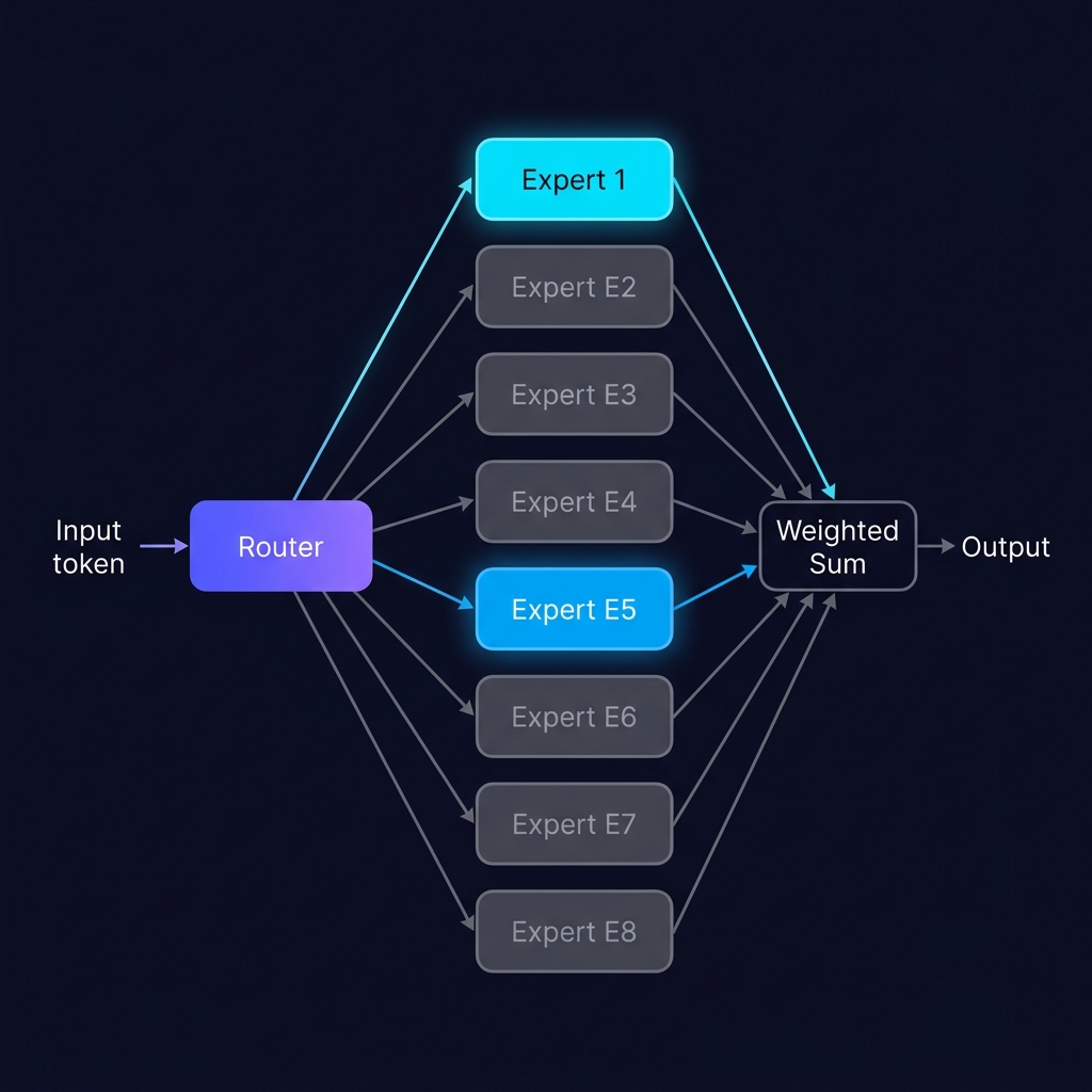
Mixtral 8×7B: 47B total, ~13B active per token

47B knowledge. 13B compute. 3.6× efficiency.

Routing is per-token

“The” → E2, E6 • “cat” → E1, E5 • “sat” → E3, E7
Each token independently picks its own K experts. Same sequence, different experts.

📄 Shazeer et al. (ICLR 2017) — “Outrageously Large Neural Networks”

Where MoE Lives in the Transformer

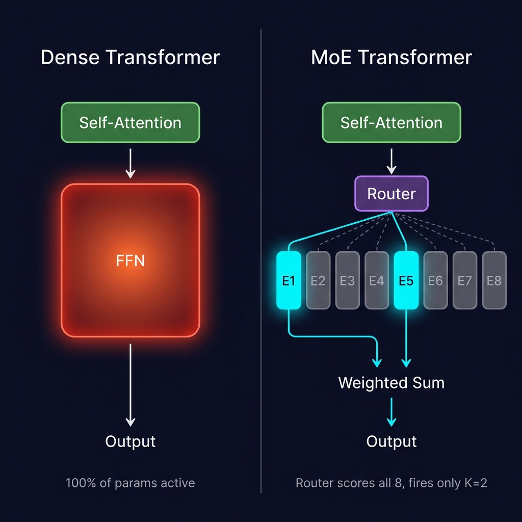
Attention stays IDENTICAL to L1. Only the FFN block changes. Everything you learned about Q/K/V still applies.

Dense vs MoE: Side-by-Side

Property	Dense 13B	MoE 47B (8×7B)
Active params	13B	~13B
Total params	13B	47B
Inference speed	Baseline	~Same
Quality	Good	Better
Memory (FP16)	26 GB	94 GB

MoE is a compute-memory trade-off. Save compute, pay with memory.

Section 2

The Router & Its Math

How tokens get routed to experts

Step 1: The Gating Function

Linear layer + softmax

$g(x) = \text{softmax}(W_g \cdot x)$

$W_g \in \mathbb{R}^{N \times D}$ • Output: probability over N experts, sums to 1

Worked Example (N=8)

Softmax output: [0.35, 0.28, 0.12, 0.08, 0.07, 0.05, 0.03, 0.02]

Expert 1 scored highest (0.35). Expert 8 lowest (0.02).

Noisy Gating (Training Only)

$H(x) = g(x) + \text{Normal}(0,\, \text{Softplus}(W_{noise} \cdot x))$

Adds noise to encourage exploration. Prevents router from converging too early. Removed at inference.

L1: same softmax as attention weights. Same function, different purpose.

Step 2: Top-K Selection

$G(x) = \text{TopK}(g(x), k)$

Mixtral: K=2 out of N=8. Top-2: [0.35, 0.28] → renormalized: [0.556, 0.444]

Experts 3–8 do ZERO computation. That’s the efficiency.

What if K = N?

You get a dense model back. No sparsity. K must be << N.

What if K = 1?

Switch Transformer (Fedus 2022). Maximum sparsity, riskier.

Step 3: Weighted Expert Output

$y = \sum_{i \in \text{TopK}} G_i(x) \cdot E_i(x)$

Each active expert runs its FFN independently. Outputs weighted by gating score and summed.

Full MoE Forward Pass

$\text{MoE}(x) = \sum_{i \in \text{TopK}(\text{softmax}(W_g x), k)} \frac{e^{w_i^T x}}{\sum_j e^{w_j^T x}} \cdot \text{FFN}_i(x)$

The Load Balancing Problem

Rich-get-richer

Without regularization → 90% of tokens go to 1–2 experts → other experts learn nothing → 75% of params wasted

A restaurant with 8 chefs but all orders go to 2 of them. You pay 8 salaries for 2 chefs’ worth of work.

Auxiliary Load Balancing Loss

$\mathcal{L}_{balance} = \alpha \cdot N \cdot \sum_{i=1}^{N} f_i \cdot P_i$

$f_i$ = fraction of tokens routed to expert i • $P_i$ = avg gating probability • $\alpha \approx 0.01$

Minimized when $f_i = P_i = 1/N$ — perfectly balanced.

Total Training Loss

$\mathcal{L}_{total} = \mathcal{L}_{task} + \mathcal{L}_{balance}$

L9: same training loop — forward, loss, backward, update. One extra term in the loss.

📄 Switch Transformers (Fedus et al., JMLR 2022)

Expert Specialization

Within one MoE layer — what do the 8 experts learn?

Token	Routed to	Pattern
`. , ; !`	E3	Punctuation & delimiters
`42 3.14 2024`	E1	Numbers & quantities
`the a an`	E6	Function words
`Bonjour café`	E2	French tokens
`def class import`	E5	Code syntax

Not exclusive — E3 handles ~70% of punctuation, not 100%. Other experts share the load. And some experts are “generalists” that fire for many token types.

Not programmed. Nobody labels tokens. Specialization emerges from training — router and experts co-evolve.

Router ≈ Semantic Router (L5)

	L5: Semantic Router	L10: MoE Router
What	Routes queries → data sources	Routes tokens → expert FFNs
How	Cosine similarity	Softmax gating
Where	Once per query	Every layer, every token
Learned?	Manual descriptions	Fully learned end-to-end

32-layer model, 100 tokens = 3,200 routing decisions. Each one is a tiny semantic router.

Section 3

MoE in Practice

Real models, deployment, and limitations

MoE Model Landscape

Model	N	K	Total	Active
Mixtral 8×7B	8	2	47B	~13B
Mixtral 8×22B	8	2	141B	~39B
DeepSeek-V2	160	6	236B	~21B
DeepSeek-V3	256	8	671B	~37B
Qwen2.5-MoE	64	8	57B	~14B
GPT-4 (rumored)	16	2	~1.8T	~220B

DeepSeek-V3: 671B total, 37B active. 18× compression.

DeepSeek Innovation: Shared Experts

$y = \underbrace{E_{shared}(x)}_{\text{always on}} + \sum_{i \in \text{TopK}} G_i(x) \cdot E_i(x)$

Shared expert handles common knowledge (grammar, reasoning) for EVERY token. Routed experts specialize in niche knowledge.

📄 Mixtral (Jiang 2024) • DeepSeek-V2 (2024) • GShard (Lepikhin 2020)

⚠ Memory vs Compute

Most common misconception about MoE

“MoE uses less memory because it’s sparse”

WRONG.

ALL N experts must be loaded. MoE saves COMPUTE, not MEMORY.

Mixtral 8×7B:
  Memory:  [E1][E2][E3][E4][E5][E6][E7][E8] = 47B loaded
  Compute: [E1][E2] only                     = 13B active

4-bit quantized Mixtral ≈ 25 GB → fits on one A100.

When to Choose MoE vs Dense

Choose MoE

Enough GPU memory available
Broad knowledge coverage needed
Best quality-to-compute ratio
General-purpose, multi-domain tasks

Choose Dense

GPU memory is tight
Edge / mobile deployment
Narrow, specific domain
Fine-tuned 7B can beat general MoE

The trend: most frontier models are MoE. Dense remains best for smaller, specialized deployments.

MoE Key Takeaways

① Replaces FFN from L1 with N experts + router. Attention stays identical.

② Router = softmax gating → top-K → weighted sum of expert outputs.

③ Load balancing loss prevents expert collapse.

④ MoE saves COMPUTE, not MEMORY. All experts must be loaded.

⑤ GPT-4, DeepSeek-V3, Mixtral all use MoE. This is the future.

☕ Break

10 minutes

Next: Multimodal — images, audio, video — any signal becomes tokens

Section 4

Multimodal: The Universal Pattern

Any signal → encoder → projection → Transformer Decoder

The Universal Pattern

ONE architecture for images, audio, video — everything

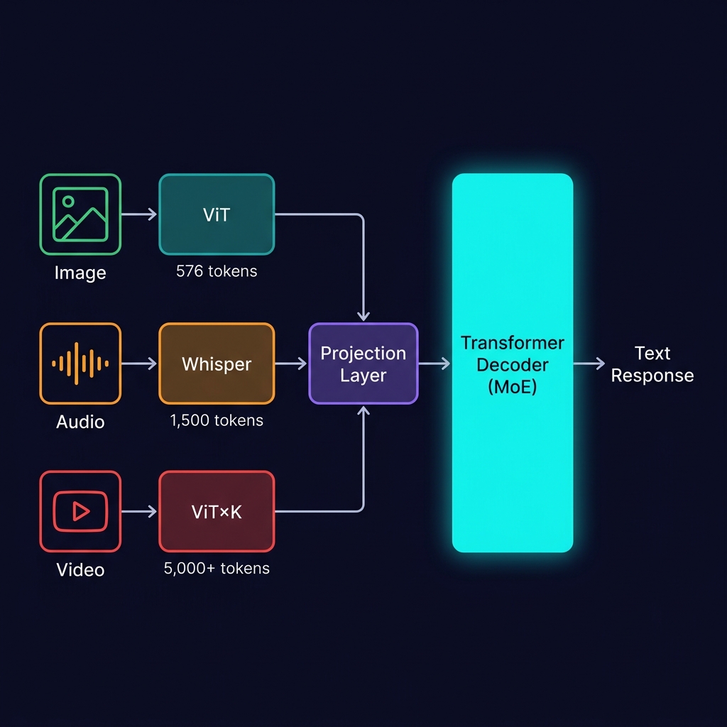
The decoder doesn’t know or care whether a token came from text, an image, or audio. They’re all vectors in the same embedding space. At this point it’s an LMM (Large Multimodal Model), not an LLM.

Modality Token Comparison

Modality	Encoder	Tokens per Unit	Cost	Models
Text	BPE tokenizer	~1.3 / word	Low	All LLMs
Image	ViT / SigLIP	~576 / image	Medium	LLaVA, Qwen-VL
Audio	Whisper encoder	~1,500 / 30s	High	Qwen2-Audio
Video	ViT + temporal	~5,000+ / 10s	Very High	Gemini, GPT-4o

Attention is $O(n^2)$. More tokens = quadratically more compute. This is the cost challenge.

🖼 From Pixels to Patches

Cutting a photo into post-it notes

Image
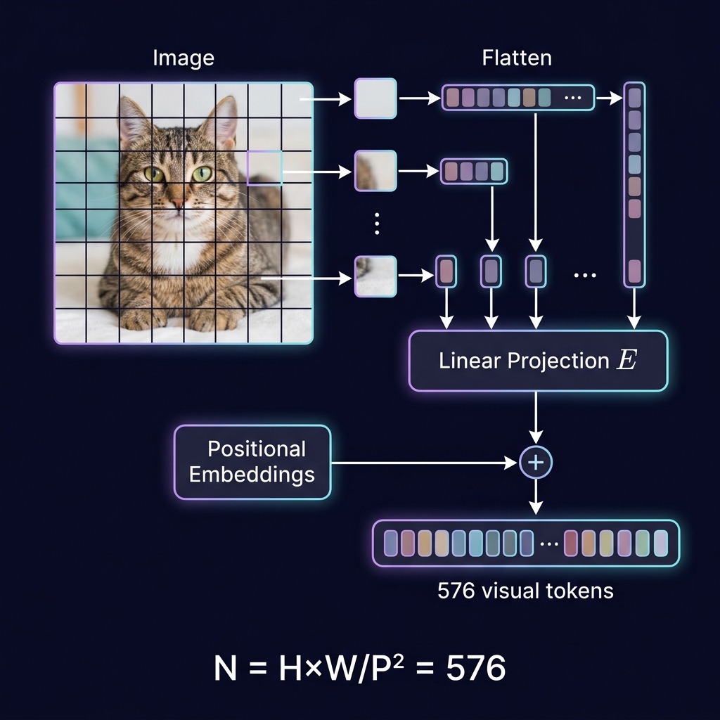
336 × 336 px

→

Cut into patches
14 × 14 px each

→

Flatten + Project
E · patch_i

→

576 tokens
+ position

$N_{patches} = \frac{H \times W}{P^2} = \frac{336^2}{14^2} = 576$

Each patch (14×14×3 = 588 values) → flattened → multiplied by E (linear projection matrix) → one token vector

L1: E is the visual equivalent of the token embedding table. Same idea — raw input → dense vector in the model’s dimension.

🖼 Bridging ViT → Decoder

ViT output dimension ≠ decoder dimension — we need a bridge

Linear Projection (LLaVA)

$h_v = W_{proj} \cdot z + b$

One matrix multiply per token.
Keeps all 576 tokens.
→ Maximum information, higher cost.

Q-Former (Qwen-VL)

$\text{Attn}(Q_{32}, K_{576}, V_{576})$

32 learnable queries attend to 576 ViT features.
Compresses 576 → 32 (18×).
→ Less info, much lower cost.

Trade-off: more tokens = better understanding but quadratically more compute ($O(n^2)$ attention).

How ViT Learns: CLIP

Contrastive learning aligns images with text — this is WHY projection works

CLIP Loss (InfoNCE)

$\mathcal{L}_{CLIP} = -\frac{1}{N} \sum_{i=1}^{N} \log \frac{e^{\text{sim}(I_i, T_i) / \tau}}{\sum_{j} e^{\text{sim}(I_i, T_j) / \tau}}$

Maximize similarity of matching pairs. Minimize non-matching. $\tau$ = learned temperature.

SigLIP (Google, used in PaliGemma)

$\mathcal{L}_{SigLIP} = -\frac{1}{N} \sum_{i,j} \log \sigma(y_{ij} \cdot s_{ij} / \tau)$

Pairwise sigmoid → more memory-efficient, scales to larger batches.

ViT was pre-trained to produce features already close to text. The projection layer just fine-tunes that alignment.

📄 CLIP (Radford, ICML 2021) • SigLIP (Zhai, ICCV 2023) • BLIP-2 (Li, ICML 2023)

🎤 Audio: From Waveform to Tokens

Whisper encoder = “ViT for audio”

Raw Audio
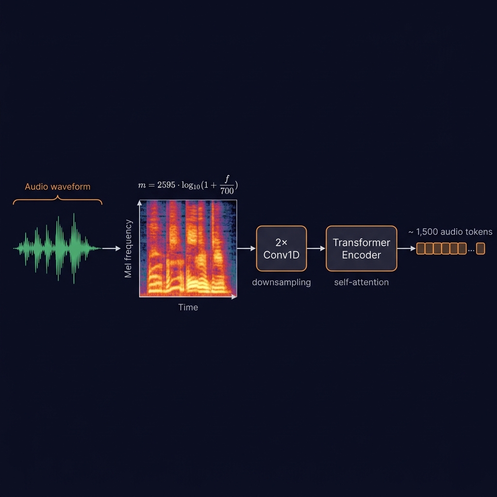
Waveform @ 16kHz

→

Mel Spectrogram
Time × Frequency

→

Conv1D × 2
Feature extraction

→

Transformer Encoder
Self-attention

→

~1,500 tokens
per 30s

Same pattern as ViT: raw signal → structured representation → encoder → tokens.

📄 Radford et al. (2023) — Whisper

🎤 Why Mel Scale?

Human hearing is logarithmic — the spectrogram must respect that

The Problem

A linear frequency axis wastes resolution. Humans perceive 100→200 Hz as the same “jump” as 1000→2000 Hz. Low frequencies (speech fundamentals) need more detail. High frequencies (hissing, noise) need less.

The Solution: Mel Scale

$m = 2595 \cdot \log_{10}\!\left(1 + \frac{f}{700}\right)$

Maps linear Hz to perceived pitch. More frequency bins for low frequencies, fewer for high — matching how we actually hear.

The mel spectrogram is a 2D image (time × frequency). Whisper’s encoder processes it like ViT processes image patches — that’s why it’s called “ViT for audio.”

🎤 Audio: Cost & Use Cases

Token Cost

30s speech = 1,500 tokens. Text query = 20–50 tokens. Audio is 30–75× more expensive.

Where Audio Multimodal Shines

Voice assistants with tone & emotion understanding
Meeting transcription + speaker ID + sentiment
Podcast/lecture Q&A directly from audio

Models

Qwen2-Audio • Gemini 2.0 • GPT-4o

🎬 Video: Temporal Sampling

Video = sequence of images. Each image is hundreds of tokens.

Video (10 seconds)

↓

Sample K frames (1fps → 10 frames)

↓

ViT per frame (576 tokens each)

↓

5,760+ video tokens

Sampling	Frames	Tokens
10s @ 1fps	10	5,760
10s @ 3fps	30	17,280
1min @ 1fps	60	34,560

Multimodal Key Takeaways

① Universal pattern: Any Signal → Encoder → Projection → Transformer Decoder. Same architecture for all modalities. It’s now an LMM, not an LLM.

② CLIP/SigLIP contrastive training is WHY projection works — ViT features are already close to text.

③ Token costs explode: text (1/word) → image (576) → audio (1,500) → video (5,000+). Attention is $O(n^2)$.

④ In MoE models, different modalities may activate different experts. MoE + multimodal = synergy.

⑤ Practical tip: always validate multimodal extraction with business rules. Never trust raw output.

Practical: Document Understanding

Traditional (5 steps)

Scan → OCR → Cleanup → NLP → Output

5 failure points

Multimodal (1 step)

Image → Model → JSON

Sees layout, structure

Uses L3 prompt techniques

Role + Task + Schema + Rules → reliable structured extraction

L4: sidesteps the “info lost in text extraction” RAG failure mode.

Section 5

Production Essentials

The 3 things you must know for serving

KV Cache & PagedAttention

$\text{KV mem} = 2 \times L \times D \times S \times B \times \text{bytes}$

Naive MHA formula. But modern models use GQA:

Grouped Query Attention (GQA)

$\text{KV}_{GQA} = 2 \times L \times \frac{D}{G} \times S \times B \times \text{bytes}$

$G = n_{heads}/n_{kv\_heads}$. Llama 3 8B: G=4 → KV cache 4× smaller (0.5 GB vs 2 GB per seq).

Traditional

~40% memory waste

PagedAttention

~4% waste → 2–4× more users

L1: K, V are the same Q/K/V projections. KV cache stores their outputs.

📄 vLLM (Kwon, SOSP 2023) • GQA (Ainslie, EMNLP 2023)

Batching & Speculative Decoding

Continuous Batching

New requests join as old finish

2–10× throughput

Speculative Decoding

$P(\text{accept}) = \min(1, p_t/p_d)$

2–3× speedup

Engine	Key Feature	Best For
vLLM	PagedAttention	GPU serving
Ollama	One-command	Dev/edge
llama.cpp	C++, quantized	Embedded

Cost Reality Check

$\text{Cost/1M tok} = \frac{\text{GPU cost/hr}}{\text{throughput} \times 3600} \times 10^6$

Self-Hosted A100

$0.28 / 1M

GPT-4o API

$2.50 / 1M

>1M tokens/day → self-hosting wins (~10× cheaper).

Course Formulas Reference

Concept	Formula	L
Attention	$\text{softmax}(QK^T\!/\!\sqrt{d_k})\!\cdot\!V$	1
Cosine Sim	$A\!\cdot\!B/(\\|A\\|\\|B\\|)$	1,4
BM25	$\Sigma\text{IDF}\!\cdot\!\text{TF}(k_1\!+\!1)/(...)$	4
RRF	$\Sigma 1/(k+\text{rank}_i)$	5
LoRA	$W'\!=\!W\!+\!(\alpha/r)BA$	9
Dense FFN	$W_2\!\cdot\!\text{ReLU}(W_1 x)$	1,10
MoE Gate	$\text{softmax}(W_g x)$	10
Noisy Gate	$g(x)+\mathcal{N}(0,\text{SP}(W_n x))$	10
MoE Out	$\Sigma G_i E_i$	10
Shared Expert	$E_{sh}(x)+\Sigma G_i E_i$	10
Balance	$\alpha N\Sigma f_i P_i$	10
CLIP Loss	$-\frac{1}{N}\Sigma\log\frac{e^{s/\tau}}{\Sigma e^{s'/\tau}}$	10
Mel Scale	$2595\log_{10}(1+f/700)$	10
ViT Patches	$HW/P^2$	10
KV Cache	$2LDSb$	10
KV (GQA)	$2L(D/G)Sb$	10
Spec Decode	$\min(1,p_t/p_d)$	10
Cost/1M	$c/(t\!\times\!3600)\!\times\!10^6$	10

Key Takeaways

① MoE replaces FFN with N experts + router. Attention stays identical. Most frontier models use it.

② Universal pattern: Any Signal → Encoder → Projection → same attention from L1.

③ Token costs explode: text (1/word) → image (576) → audio (1,500) → video (5,000+).

④ KV cache + PagedAttention = serving bottleneck + solution.

⑤ Every lecture maps to a production component. Start simple, measure, iterate.

Questions?

10 lectures — from attention to multimodal MoE systems.

Kamyar Zeinalipour — Zucchetti LLM Course

Modern LLM Architectures& Multimodal AI